


When we first built Scalyr, we focused on making it fast and easy to extract answers from logs. Over the years, as we add capabilities, we’ve maintained that focus on simplicity and speed. We based our search capabilities on a straightforward filtering language that is easy to learn and easy to use, in conjunction with a carefully chosen set of UI-based tools for visualization and exploration that has served us very well. It covers the vast majority of use cases, and our customers love it. We’ve seen some impressive adoption rates – more than 50% at some organizations, which is unheard of for this type of tool.
Older log management solutions grew up with complex query languages, including huge libraries of “commands” to manipulate and visualize data. These complex languages make advanced tasks possible, but are difficult and cumbersome even for everyday tasks. Only a handful of users ever really know how to use the language, and they typically have to undergo extensive training and certification in order to be productive.
While focusing on speed and ease of use has paid off, we’ve always known that there are advanced use cases that require a more powerful query language, and that we would eventually want to address those use cases. At the same time, we wanted to avoid the overwhelming complexity that legacy solutions have accumulated over the years. With the benefit of experience, we were in a position to create a clean-sheet design that supports powerful data manipulation with a relatively simple language. The result is PowerQueries: a new set of commands for transforming and manipulating data on the fly, combining Scalyr’s traditional speed and ease of use with the power of composable operations. In this article, we’ll talk about how we were able to accomplish this without sacrificing performance.
What’s powering PowerQueries
To ground the discussion, let’s work from an example. Imagine that you’re running a tax accounting service. Your software has to be customized according to the tax laws in each state, and so you want to monitor for service quality in each state. The information you need is in your access logs, which might look like this (simplified):
                  34.205.61.122 GET /taxForm?state=CA 200
                  54.73.130.161 GET /taxForm?state=NY 502
                  18.234.28.209 GET /taxForm?state=TX 200
                  52.199.254.64 GET /taxForm?state=CA 200
                  13.251.118.78 GET /taxForm?state=MI 503
                  169.47.29.230 GET /taxForm?state=WA 200
                  18.234.28.103 GET /taxForm?state=TX 200
                  52.199.44.149 GET /taxForm?state=NY 502
                  11.200.118.62 GET /taxForm?state=OH 200
                  47.123.29.100 GET /taxForm?state=NY 200
To detect problems, you might count the number of errors in each state. However, that’s going to be thrown off by population size – big states like California and Texas will have more traffic, which will naturally lead to more errors, even if nothing unusual is happening. What you really want to know is the percentage of errors in each state. PowerQueries support that kind of analysis. Here’s a basic solution:
tier="formServer" log="access" page="/taxForm"
| group total_requests = count(),
        errors = count(status >= 500 && status <= 599)
     by state
| let error_rate = errors / total_requests
This query finds all access log records for your tax form server, groups them by state, counts the number of successful and failed requests, and computes the error percentage. For extra credit, we might add commands to discard states with a minimal error rate or with insufficient traffic to compute meaningful statistics, and then sort by descending error rate:
tier="formServer" log="access" page="/taxForm"
| group total_requests = count(),
        errors = count(status >= 500 && status <= 599)
     by state
| let error_rate = errors / total_requests
| filter total_requests >= 1000 && error_rate > 0.0001
| sort -error_rate
There are a significant number of processing steps here, and real-world queries can get considerably more complex, with multiple rounds of text parsing, arithmetic, string manipulation, grouping and filtering. When operating on terabytes of log data, this rapidly becomes expensive. Three things make PowerQueries fast:
- We designed the data pipeline to apply the simplest possible processing to the largest amounts of data.
- We leveraged Scalyr’s massive multi-tenant processing cluster.
- We carefully tuned the performance-critical components of the system.
Inverted data pipeline design
Let’s consider what takes place when executing the query above. First, from the collective mass of log data, we identify just the access logs for the tax form server:
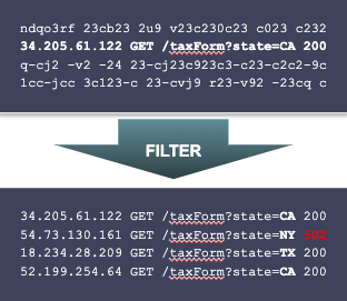
Next, we group the matching records by state, counting total and failed requests:
There are still several processing steps remaining. However, from a performance standpoint, the hard work is already done. From this point forward, we’re working with a tiny amount of data. We’ve reduced millions or billions of logs records to a table with just 50 rows, one for each state. So when we’re worrying about performance, we focus on the first two steps – filtering and grouping.
Fortunately, filtering is something Scalyr is already very, very good at. Every PowerQuery begins with a filtering stage to identify the relevant logs. This is the exact same problem as the initial filtering stage of any other Scalyr query, and we’ve built an extremely efficient engine for that. PowerQueries use that engine to perform the initial filtering stage and identify the log records which are used by the query. This is enhanced by an initial planning step that identifies filtering rules which can be executed up front, even if they’re not on the first line of the query.
Massive multi-tenant processing
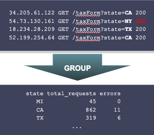
Much of Scalyr’s performance comes from the distributed, multi-tenant architecture. Log data is distributed across a large number of storage-and-compute nodes, each of which participates in query execution. The engine supports pluggable processing stages, so we were able to implement the PowerQuery grouping stage as a plugin module that executes on every node in parallel:
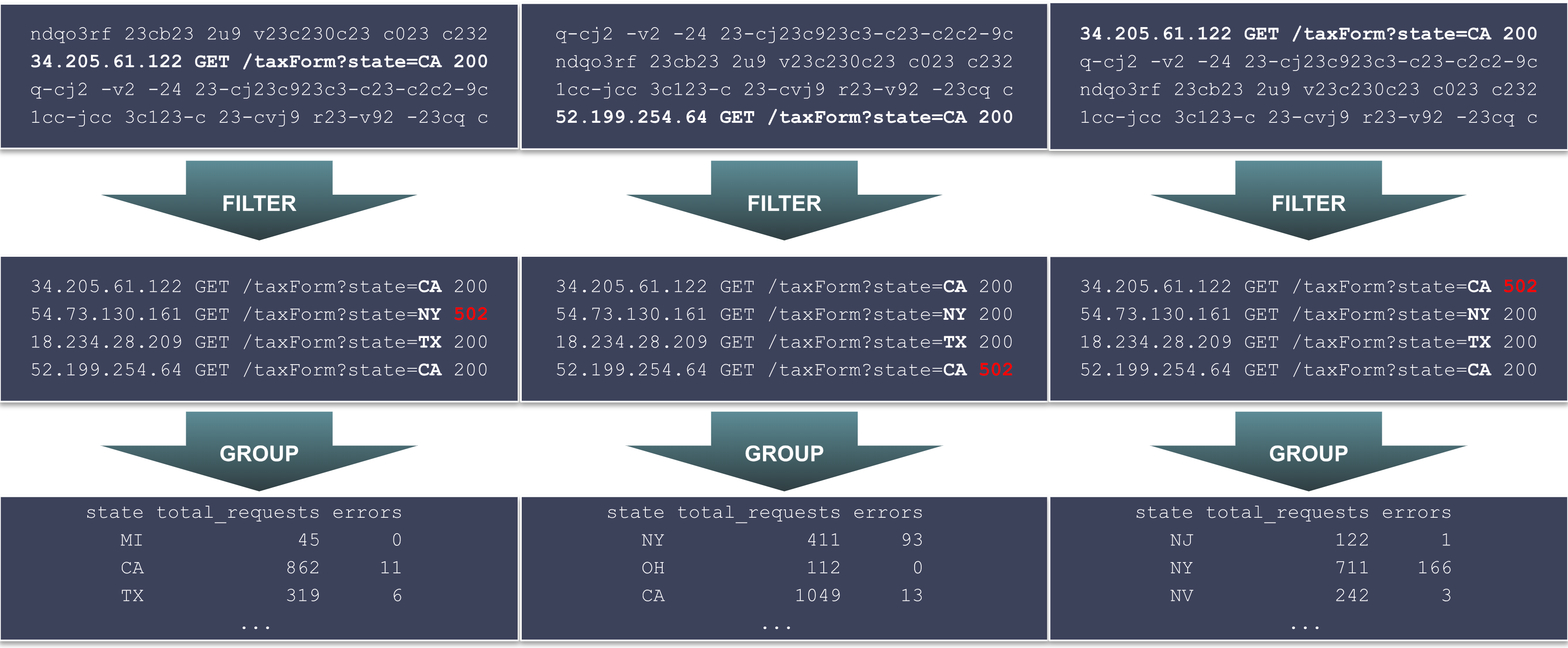
Each node produces an intermediate grouping table, listing (in this example) state-by-state statistics for all logs stored on that node. These intermediate results are then sent back to a central server, combined, and the final processing stages of the query are executed:
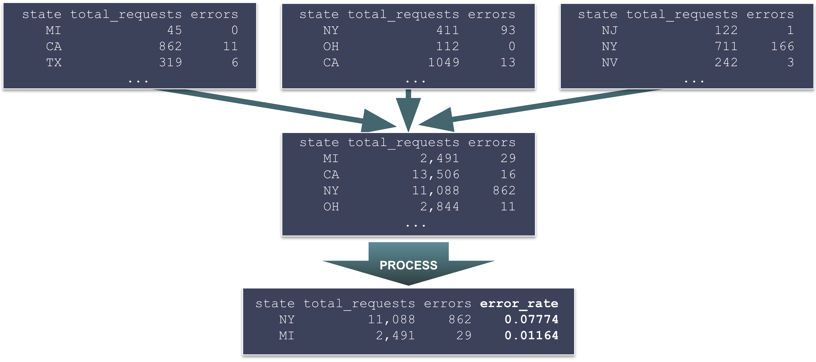
This works well because the stage that processes the largest amount of data – the initial filter step – uses our existing, highly tuned search engine. The next stage – grouping – is more complex, but is still able to rely on the brute power of our massive processing cluster. The final stages are less optimized, but work with a much smaller amount of data. In round numbers, the amount of data processed at each stage might look something like this:
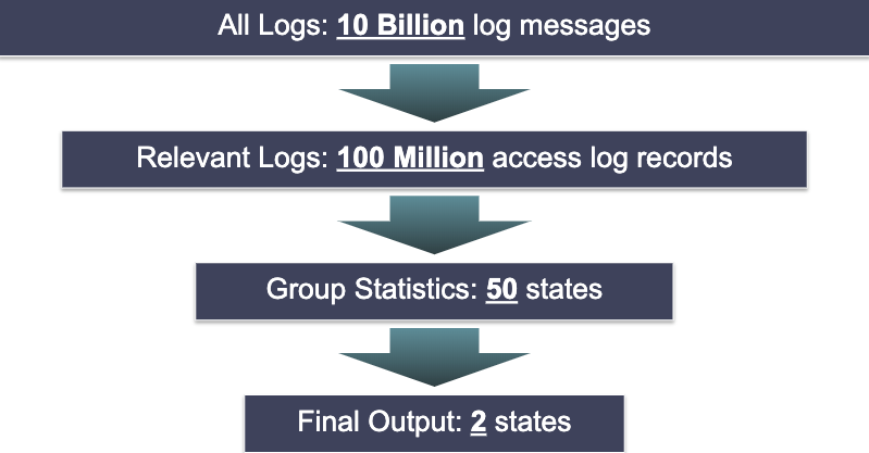
By focusing our optimization efforts on the first two stages, we’re able to achieve high performance without overly burdening the implementation of the later, more sophisticated processing steps.
Tuning performance-critical components
While the largest data volume is processed by our existing search engine, the second stage – where we process and group the matching log records – also needs to handle large amounts of data. Let’s think about the work that happens for each log message matching the initial filter. In our sample query, this corresponds to the second command:
group total_requests = count(),
        errors = count(status >= 500 && status <= 599)
     by state
Breaking it down, here’s what has to happen for each message:
- Retrieve the “status” field. (DataSet parses logs at ingestion time, so the HTTP status will already have been extracted from the access log and stored in numeric form.)
- Compare status to 500.
- Compare status to 599.
- Merge the results of the previous two steps, to determine whether status is in the range 500-599, which indicates a server error.
- Retrieve the “state” parameter from the URL. (Again, this parameter will have been parsed at ingestion time. If not, we could use the “parse” command to extract it now.)
- In the internal table where we assemble query results, find the row corresponding to the value in the state field.
- Increment the value in the total_requests column.
- If status was in the range 500-599, then increment the value in the errors column.
That’s a lot of steps! To efficiently perform this sort of processing, we built a lightweight virtual machine. Programs for this virtual machine preallocate all of their storage, so no memory allocation is taking place as we process events. As a result, performance is both fast and predictable.
Another important point was the design of the data structure that aggregates values by grouping keys – the “table where we assemble query results”. In our example, this table has only a handful of columns, and 50 rows. However, some queries might have a dozen columns, tens of thousands of rows, and perform billions of insertions and updates. For each query, the engine creates a row-major memory layout which is customized according to the number and types of intermediate values generated by that query. The row-major format minimizes cache misses when updating multiple columns for a single grouping key; and customizing the layout for each query allows memory allocation to be done in large, efficient blocks.
